Student's t-distribution comparing means

Introduction

The student's t-distribution is used for statistical inferences based on measured means of normally distributed populations. I will briefly summarize how to use the student's t-distribution to determine the probability that the means of two distributions are different. Because the distribution is defined in terms of $\Gamma$ functions, which are not available in all languages (e.g. versions of C++ prior to C++11), I will derive a good approximation that is easy to evaluate.

Welch's t-test

A t-test gives a t-value that basically describes how many standard deviations outside of the mean one distribution is from another. We will assume that we have taken samples of a relatively larger population. Give two distributions indexed by the subscript $i$, the measured mean is $\mu_i$, the measured standard deviation is $\sigma_i$, and the number of samples taken is $n_i$. From these statistics, we define the standard error of the mean as $e_i = \sigma_i / \sqrt{n_i}$ and the degrees of freedom as $\nu_i = n_i - 1$.

From these statistics of the individual distributions, we can find the relation between the means using Welch's t-test. Welch's t-test defines the t-value between the distributions as $$ t_{12} = \frac {|\mu_1-\mu_2|} {\sqrt{e_1^2+e_2^2}} ,$$ with degrees of freedom equal to $$ \nu_{12} = \frac {(e_1^2+e_2^2)^2} { \frac {e_1^4} {\nu_1} + \frac {e_2^4} {\nu_2} } .$$

With these descriptors of the difference between distributions, we can now determine the probability that the distribution means $\mu_1 = \mu_2$ are the same. This is a two-tailed test because the means could be different either by $\mu_1 < \mu_2$ or $\mu_1 > \mu_2$. Given the cumulative distribution function (CDF) of the student's t-distribution $F_{student}$, we can find the probabilities of the means being the same $p_{same}$ or different $p_{different}$ as $$ p_{same} = 2 F_{student}(-t_{12}, \nu_{12}) $$ $$ p_{different} = 1 - p_{same} .$$

Student's t-distribution

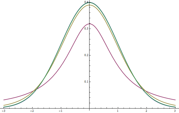
The student's t-distribution $f_{student}$ is defined as $$ f_{student}(t,\nu) = \frac 1 {\sqrt \nu B(\frac 1 2, \frac \nu 2)} \left( 1 + \frac {t^2} \nu \right) ^ {- \frac {\nu + 1} 2} ,$$

where $$ B(a, b) = B(b, a) = \frac {\Gamma(a)\Gamma(b)} {\Gamma(a+b)} = \int_0^1 t^{a-1} (1-t)^{b-1} ~dt .$$

As $\nu$ increases, the student's t-distribution approaches the normal distribution, and is equal to the normal distribution in the limit as $\nu \rightarrow \infty$. I show a graph with different values of $\nu$ in Figure #1.

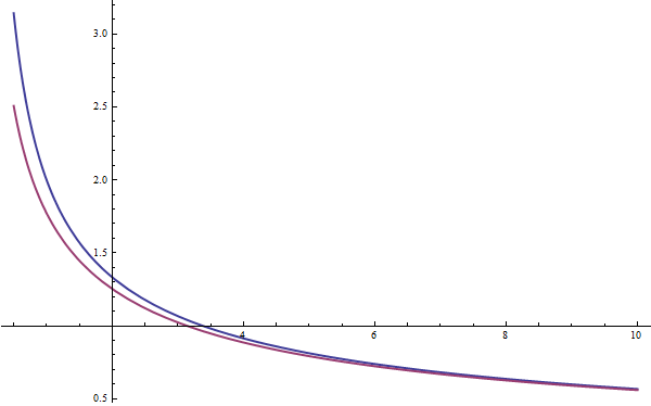
Our problem is that $B$ is somewhat difficult to compute because there is no closed-form expression to evaluate $\Gamma$. By Stirling's approximation when $a$ is large and $b$ is fixed, $B(a,b) \approx \Gamma(b) a^{-b}$. This means we can use the approximation that $$ B\left(\frac 1 2, \frac \nu 2 \right) \approx \Gamma\left(\frac 1 2\right) \left(\frac \nu 2\right)^{-\frac 1 2} = \frac {\sqrt \pi} {\sqrt \nu}.$$

I plot $B$ in blue and this approximation in purple over the domain of $\nu \in [.5, 10]$ in Figure #2. You can see that as $\nu$ increases the approximation converges, but that at low values the approximation is somewhat off.

In Figure #3 I plot $B$ divided by the approximation in blue. In other words, the blue line is the factor by which I must multiply the approximation in order to get $B$.

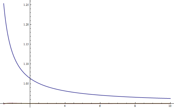
This ratio shown in blue looks somewhat like a rational function, of the form $$ 1 + \frac c \nu ,$$ where $c$ is some scaling constant. By numerically minimizing the squared error over the domain $\nu \in [.5, 100]$, I found the optimal $c = 0.12756096170787165$. It is worth noting that, by construction, as $\nu \rightarrow \infty$ my corrective factor approaches one, which is good because in the limit the original approximation converges to $B$. In Figure #3 I show my new approximation with the rational scaling factor in purple. The error is much lower than before, and it is difficult do see that the purple line is different from one at this scale, so I show a zoomed version of the same graph in Figure #4.

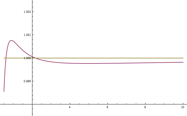
In the worst case, when there are very low numbers of samples, this approximation is off by about 1 in 1000 and is even better for more reasonable numbers of samples. Plugging this approximation of $B$ into the definition of $f_{student}$ we find that $$ f_{student}(t,\nu) \approx \frac {0.3989422804014327 \nu} {0.2551219234157433 + \nu} \left( \frac {\nu + t^2} \nu \right) ^ {-.5 \nu - .5} .$$

This can be written in C++ code as:

double student_pdf(double t, double n)
{
    return (0.3989422804014327*n*pow((n + t*t)/n,-0.5 - 0.5*n))
        /(0.2551219234157433 + n);
}

Student's t-distribution CDF

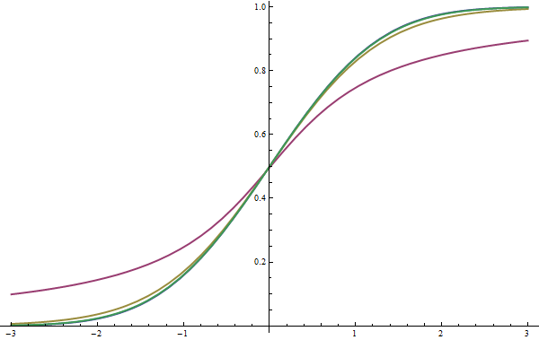
The last step required to evaluate the probability of means being the same or different is to evaluate the CDF of the student's t-distribution. The CDF is defined as $$ F_{student}(t,\nu) = \int_{-\inf}^t f_{student}(x,\nu) ~dx.$$ I have not looked much into approximating this function with a closed-form expression. Instead, I perform numeric integration. Numeric integration works quite well, because $f_{student}$ is smooth and flat, especially when evaluated far from the origin. I show some examples of the CDF for different values of $\nu$ in Figure #5. Again, as $\nu$ increases, $F_{student}$ approaches $F_{normal}$.

A problem with numerically integrating the value of the CDF that I wrote above is that it requires integrating from $-\infty$, which is obviously not possible. One solution that people will use is to integrate from a starting value $t_0$ that is sufficiently negative that the integral $$ \int_{-\infty}^{t_0} f_{student}(x,\nu) ~dx \approx 0$$ so that $$ \int_{t_0}^{t} f_{student}(x,\nu) ~dx \approx F_{student}(t,\nu).$$

The problem with this approach is that when $\nu$ is small, the tails of the function are relatively large compared to in the normal distribution, so it is somewhat difficult to choose an appropriate $t_0$, and it is best to be safe by using a very negative starting value such as $t_0 = -100$. This has two problems. First, it does not provide a very nice theoretical bound on the error. Second, we must evaluate the integral over a very large domain of mostly zero values, whereas we typically only want to find probabilities for small $t$, such as $|t| < 10$.

A better approach is to directly evaluate the probability of the means being different as $$ p_{different} = \int_{-t}^{t} f_{student}(x,\nu) ~dx = 2\int_{0}^{t} f_{student}(x,\nu) ~dx .$$

The C++ code to numerically evaluate this integral is given below.

double student_prob_different(double t, double n)
{
    if (t <= 0)
        return 0;

    int steps = (int)ceil(t * 100);
    double dt = t / steps;

    double sum = 0;
    for (double x = dt*.5; x < t; x += dt)
        sum += student_pdf(x, n);

    sum *= 2 * dt;
    return sum;
}

double student_prob_same(double t, double n)
{
    return 1 - student_prob_different(t, n);
}